A Derivation of 2D Semi-Implicit MPM

Yu Zhang

April 2023

Introduction

The most common implicit methods of MPM are energy-based solvers, often employing matrix-free methods (like PCG) to avoid the explicit construction of stiffness matrices. To help readers better understand the details of the stiffness matrix, we provide a full derivation for a 2D semi-implicit method, and give the explicit form of the stiffness matrix.

What is Semi-Implicit Time Integration?

This section introduces explicit, semi-implicit, and fully implicit methods for time integration.

Explicit Time Integration

In physical simulations, there are various methods to discretize time integration. The simplest one is explicit time integration, such as the symplectic Euler method: $$ \begin{aligned} \mathbf{v}^{n+1} &= \mathbf{v}^{n} + \frac{\mathbf{f}^n}{m} \Delta t \\ \mathbf{x}^{n+1} &= \mathbf{x}^{n} + \mathbf{v}^{n+1} \Delta t \end{aligned} \\ $$ Where the superscript $n$ represents the value of the variable at discrete time step $n$, and superscript $n+1$ represents the value at time step $n+1$.

Implicit Time Integration

Implicit methods typically require solving a system of equations, such as the backward Euler method: $$ \begin{equation} \begin{aligned} \mathbf{v}^{n+1} &= \mathbf{v}^{n} + \frac{\mathbf{f}^{n+1}}{m} \Delta t \\ \mathbf{x}^{n+1} &= \mathbf{x}^{n} + \mathbf{v}^{n+1} \Delta t \end{aligned} \end{equation} $$ Based on these two equations, fully implicit and semi-implicit methods can be introduced.

Fully Implicit Time Integration

Energy-based solver is a type of fully implicit method: $$ \begin{aligned} E(\mathbf{v}) = \frac{1}{2} m ||\mathbf{v}-\mathbf{v}_n||^2 + e(\mathbf{x}_n + \Delta t \mathbf{v}) \end{aligned} $$ This fully implicit method can be solved using the Newton's method.

Semi-Implicit Time Integration

The semi-implicit method we are going to introduce is also based on the equation (2.2). We approximate $f_{n+1}$ using the first-order Taylor expansion: $$ \begin{aligned} \mathbf{f}^{n+1} &= \mathbf{f}(\mathbf{x}^n + \Delta t \mathbf{v}^{n+1}) \\ &= \mathbf{f}^n + \Delta t \mathbf{v}^{n+1} \frac{\partial \mathbf{f}}{\partial \mathbf{x}} (\mathbf{x}^n) \end{aligned} $$ This is the semi-implicit method.

Why Use Semi-Implicit Time Integration?

In explicit time integration, when the stiffness is large (the simulation time step remains constant), the system can experience overshooting. Velocities can oscillate wildly, possibly diverging to positive or negative infinity, leading to simulation failure. In explicit methods, the only way to address this issue is by reducing the time step, but very small time steps can severely degrade simulation performance. Implicit methods effectively resolve this problem. We choose the semi-implicit approach because, within the typical material stiffness range, it is sufficient to support stable simulations with larger time steps without the need for a fully implicit method.

Derivation of the Semi-Implicit Time Integration

From the formula, it can be seen that the most crucial step is to solve for $\frac{\partial \mathbf{f}}{\partial \mathbf{x}} (\mathbf{x}^n)$. In some numerical methods, this term can be avoided through implicit construction (e.g., using the conjugate gradient method). To the best of the author's knowledge, in most of currently available MPM implementations on the internet, the CG method is used to avoid the explicit calculation of this term, and no one has provided its explicit form. Today, we will explicitly derive it to help everyone's understanding. Our general approach is to break down this relatively complex formula into several independent parts and derive each part separately, making it easier to comprehend. In the MPM framework, after discretization, this term can be written as: $$ \frac{\partial \mathbf{f}_i}{\partial \mathbf{x}_j} (\mathbf{x}^n) = \frac{\partial^2 e}{\partial \mathbf{x}_i \partial \mathbf{x}_j} (\mathbf{x}^n) = - \sum_p \frac{\partial^2 e_p}{\partial \mathbf{x}_i \partial \mathbf{x}_j} (\mathbf{x}^n) = - \sum_p V_p \frac{\partial^2 \Psi_p}{\partial \mathbf{x}_i \partial \mathbf{x}_j} (\mathbf{x}^n) $$ Here, subscripts $i$ and $j$ represent grid cell indices, and subscript $p$ represents particle indices. From the above equation, it can be seen that we only need to calculate the contribution of each particle to this term. The most crucial part to come is the derivation of $\frac{\partial^2 \Psi_p}{\partial \mathbf{x}_i \partial \mathbf{x}_j} (\mathbf{x})$, where, for convenience, we omit the parameter $\mathbf{x}$. According to the chain rule: $$ \frac{\partial^2 \Psi_p}{\partial \mathbf{x}_i \partial \mathbf{x}_j} = \frac{\partial \Psi_p}{\partial \mathbf{F}_p} : \frac{\partial^2 \mathbf{F}_p}{\partial \mathbf{x}_i \partial \mathbf{x}_j} + \frac{\partial^2 \Psi_p}{\partial \mathbf{F}_p \partial \mathbf{F}_p} : \frac{\partial \mathbf{F}_p}{\partial \mathbf{x}_i} : \frac{\partial \mathbf{F}_p}{\partial \mathbf{x}_j} $$ Here, the symbol $:$ represents the tensor contraction operation, which is the inner product of tensors along two dimensions. For the sake of clarity, I have not written the corresponding indices, but when implementing the contraction, be careful not to select the wrong dimensions. Next, we will continue the derivation using MLS-MPM and the fixed-corotated model as examples. For MLS-MPM, the first term in the above equation can be removed because $\frac{\partial^2 \mathbf{F}_p}{\partial \mathbf{x}_i \partial \mathbf{x}_j}$ has a value of 0. Now, we will prove this. In MLS-MPM, the deformation gradient $\mathbf{F}_p$ has the following form: $$ \mathbf{x}_i = \mathbf{x}_i^n + \Delta t \mathbf{v}_i \\ \mathbf{C}_p(\mathbf{x}) = \frac{4}{\Delta \mathbf{x}^2} \sum_i w_{ip}^n \mathbf{v}_i (\mathbf{x}_i^n - \mathbf{x}_p^n)^T \\ \mathbf{F}_p(\mathbf{x}) = (\mathbf{I} + \Delta t \mathbf{C}_p) \mathbf{F}_p^n $$ Calculations show that $\frac{\partial^2 \mathbf{F}_p}{\partial \mathbf{x}_i \partial \mathbf{x}_j} = 0$. In fact, this conclusion also holds for Traditional MPM. So, we've got $$ \frac{\partial^2 \Psi_p}{\partial \mathbf{x}_i \partial \mathbf{x}_j} = \frac{\partial^2 \Psi_p}{\partial \mathbf{F}_p \partial \mathbf{F}_p} : \frac{\partial \mathbf{F}_p}{\partial \mathbf{x}_i} : \frac{\partial \mathbf{F}_p}{\partial \mathbf{x}_j} $$

Derivation of $\frac{\partial^2 \Psi_p}{\partial \mathbf{F}_p \partial \mathbf{F}_p}$

This term is only related to the constitutive model and is independent of the algorithm. Next, we will use the fixed-corotated model as an example to derive it. For a rotationally invariant and isotropic constitutive model, we can establish the relationship between the components of $\mathbf{F}_p$ and $\Psi_p$ using the eigenvalues $s_1, s_2$ of the deformation gradient $\mathbf{F}_p$ and their rotational components $u_1, v_1$. In the case of 2D, we give a Mathematica script to calculate this term. This script is based on a similar Mathematica script provided in Professor Chenfanfu Jiang's MPM course. However, Professor Jiang's original program did not directly meet our needs; it calculated the value of this term when $u_1 \rightarrow 0, v_1 \rightarrow 0$. Here, we provide the modified program directly:

var ={ s1 , s2 , u1 , v1 } ;
S=DiagonalMatrix [ { s1 , s2 } ] ;
U= { { Cos [ u1 ] , - Sin [ u1 ] } , { Sin [ u1 ] , Cos [ u1 ] } } ;
V= { { Cos [ v1 ] , - Sin [ v1 ] } , { Sin [ v1 ] , Cos [ v1 ] } } ;
F=U. S . Transpose [V ] ;
dFdS=D[ Flatten [ F ] , { var } ] ;
dSdF= Inverse[ dFdS] ;
(* fixed corotated model: mu and la are Lamé coefficients *)
Phat=DiagonalMatrix [ { 2*mu*(s1-1)+la*(s1*s2-1)*s2,  2*mu*(s2-1)+la*(s1*s2-1)*s1} ] ;
P=U. Phat . Transpose [V ] ;
dPdS=D[ Flatten [ P ] , { var } ] ;
dPdF=Simplify[ dPdS . dSdF ] 

After calculating, the result looks something like this:

I’ve already copied this result for you, and the code is available here.

Derivation of $\frac{\partial \mathbf{F}_p}{\partial \mathbf{x}_i} $

This term is independent of the constitutive model and depends on the choice of algorithm. For MLS-MPM and Traditional MPM, the results of this term are different. The derivation of this term is relatively straightforward. Here, we use MLS-MPM as an example, and other MPM methods like Traditional MPM follow a similar approach. For convenience, we also use Mathematica for the derivation.

(*constants*)
id=IdentityMatrix[2];
Fp = { {F00, F01},{F10, F11} };
wi={wi0, wi1};
wj={wj0, wj1};
xp = {xp0, xp1};
xxi0 = {xii0, xii1};
xxj0 = {xjj0, xjj1};

(*variables*)
xi = {xi0, xi1};
v = (xi-xx0)/t;
xj = {xj0, xj1};
vj = (xj-xxj0)/t;

factor=4*invdx*invdx;

F =FullSimplify[ (id+t*factor*(Outer[Times,v,xx0-xp]*wi + Outer[Times,vj,xxj0-xp]*wj)).Fp];
dFdxi = FullSimplify[D[Flatten[F],{xi}]]

The result looks something like this:

Assembly

Now that we have $\frac{\partial^2 \Psi_p}{\partial \mathbf{F}_p \partial \mathbf{F}_p}$ and $\frac{\partial \mathbf{F}_p}{\partial \mathbf{x}_i}$, we can calculate $\frac{\partial^2 \Psi_p}{\partial \mathbf{x}_i \partial \mathbf{x}_j}$ in the code as follows: $$ \frac{\partial^2 \Psi_p}{\partial \mathbf{x}_i \partial \mathbf{x}_j} = \frac{\partial^2 \Psi_p}{\partial \mathbf{F}_p \partial \mathbf{F}_p} : \frac{\partial \mathbf{F}_p}{\partial \mathbf{x}_i} : \frac{\partial \mathbf{F}_p}{\partial \mathbf{x}_j} $$ If you want to skip the two separate steps above and directly obtain the final result $\frac{\partial^2 \Psi_p}{\partial \mathbf{x}_i \partial \mathbf{x}_j}$ in one step, it is also possible. In Mathematica, you can use the following code to obtain its result in one step (using $K$ to represent this term in the code):

dFdxi = FullSimplify[D[Flatten[F],{xi}]]
dFdxj = FullSimplify[D[Flatten[F],{xj}]];
A = TensorContract[TensorProduct[dPdF,dFdxi],{ {2,3} }];
K = TensorContract[TensorProduct[A,dFdxj],{ {1,3} }]

Although skipping these separate two steps can also derive the final formula, I personally do not recommend doing so because separately calculating each term is more convenient for error localization and makes it easier to replace each module with other constitutive models or MPM algorithms.

Experimental Results

In our implementation, the solid density is set to 1, so there is a scaling factor of 1000 when the Young’s modulus E in the program corresponds to material stiffness in real life. For example, if we set E=1e4 in our program, it is equivalent to a material with a Young’s modulus of 1e7 in the real world.

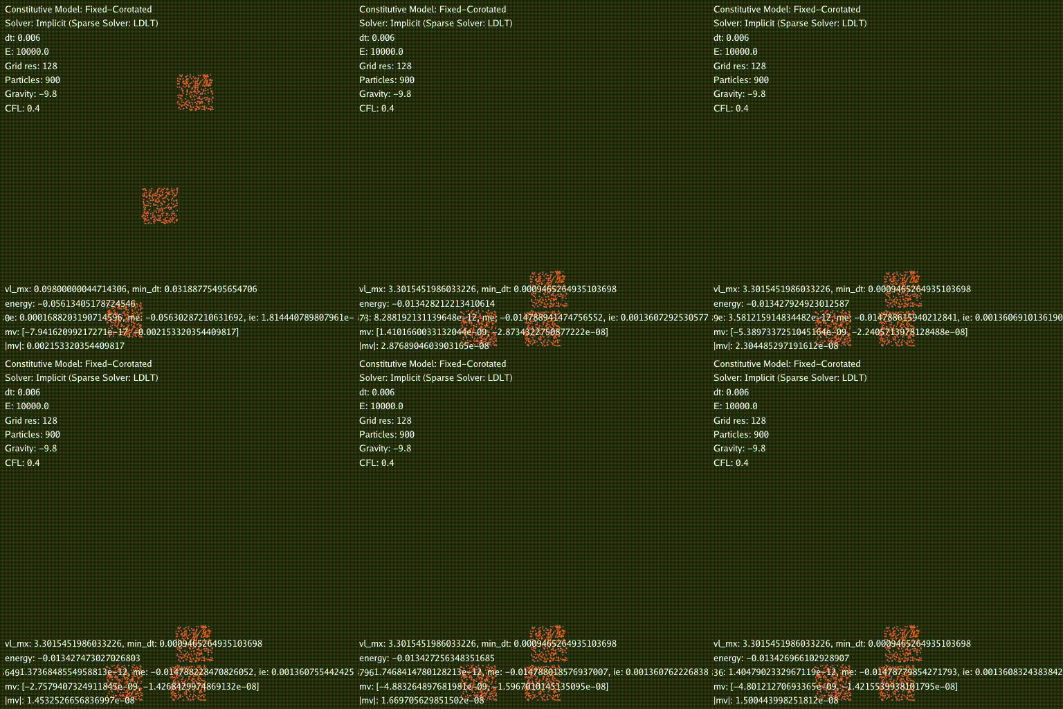
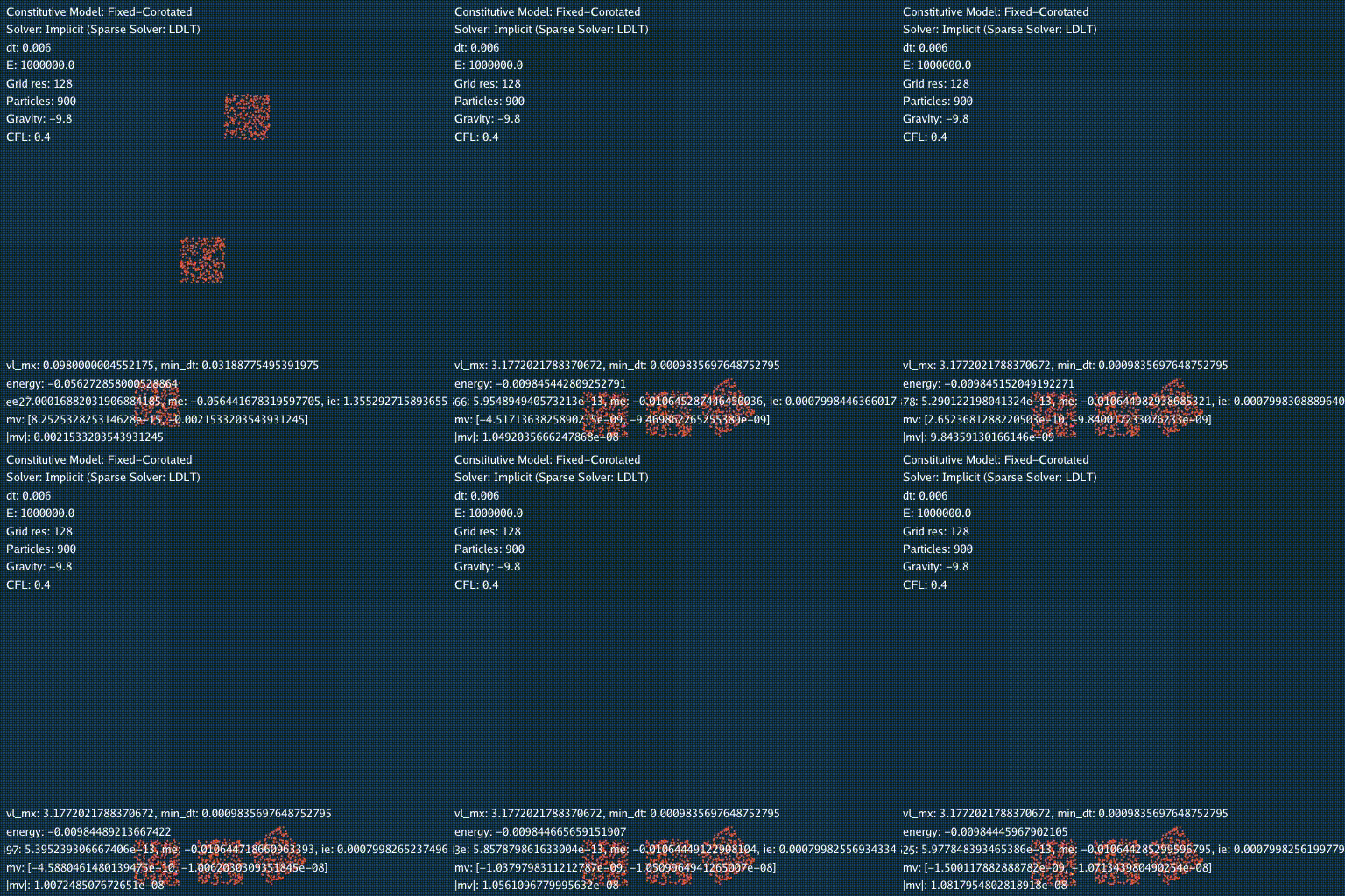
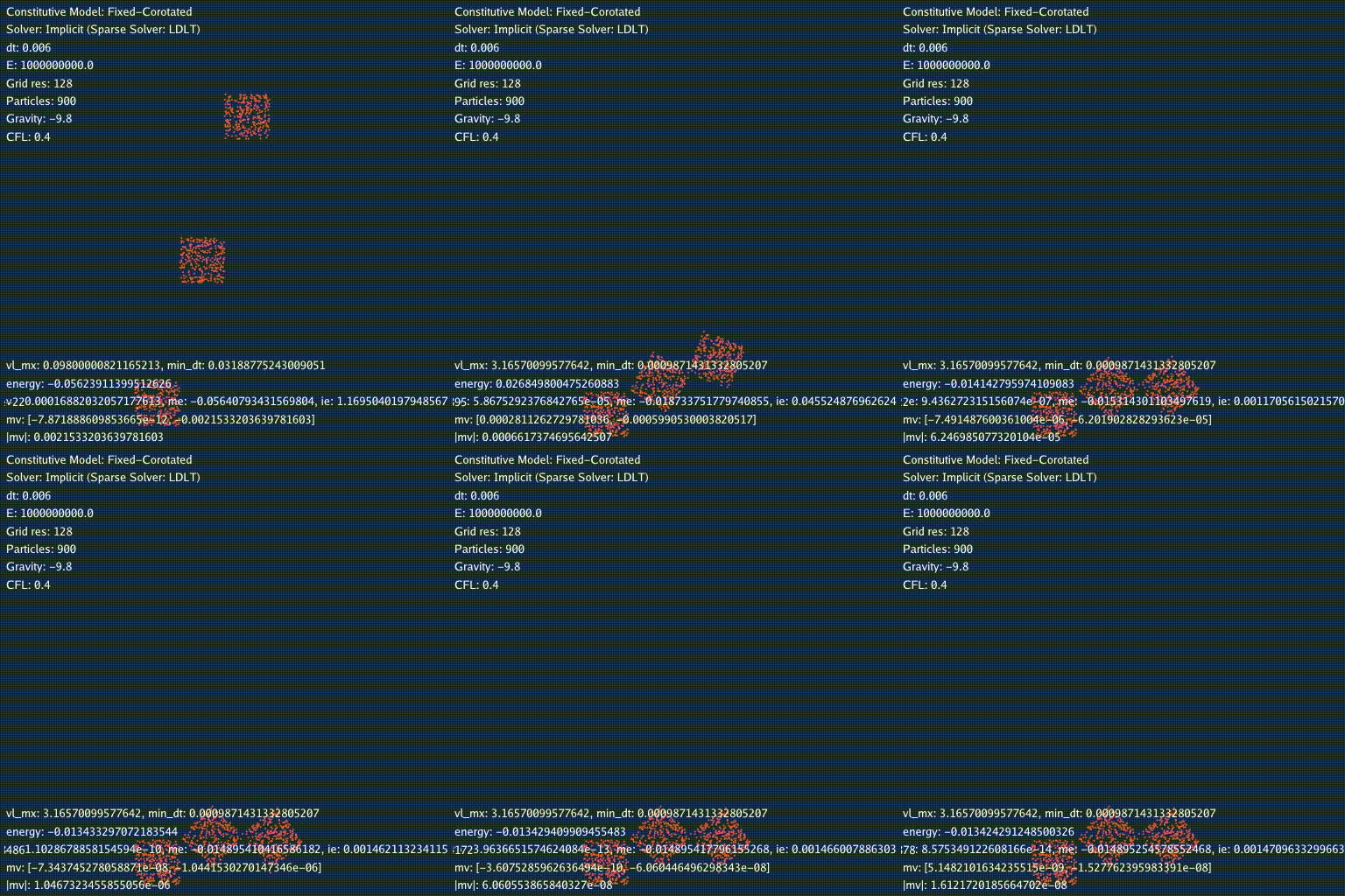
Regarding the time step, we control the CFL coefficient to be 0.4, which ensures that particles do not move more than 0.4 grid cell sizes within each time step. Based on this, we demonstrate the simulation of hard rubber, bone, and diamond under relatively large desired time steps (1e-2). Note: the actual time step here is calculated as min(CFL-allowed time step, desired time step). The experimental results are as follows:

In Figure 1, E = 1e4, which is equivalent to a Young’s modulus of 1e6 for hard rubber. In Figure 2, E = 1e6, which is equivalent to a Young’s modulus of 1e9 for bone. In Figure 3, E = 1e9, which is equivalent to a Young’s modulus of 1e12 for diamond.

Limitations of the Semi-Implicit Method

Common Issues with Implicit Methods

Implicit methods share a common problem: they introduce additional numerical damping (because the algorithm is not “symplectic”). The manifestation of this issue is that when the time step is large, objects appear to be more “viscous”. As seen in the simulation scenario of a diamond, under large time steps and stiffness, the results produced by implicit methods become unacceptable. For objects with such stiffness, simulation can only be achieved by reducing the time step or using a rigid-body physics engine.

Another reason is that temporal discretization is essentially a first-order Taylor expansion $\mathbf{x}^n + \Delta t \mathbf{v}$ in time step $\Delta t$, and Taylor expansion is inaccurate when the time step $\Delta t$ is large. Therefore, it may fundamentally fail to simulate the correct behavior.

Issues with Semi-Implicit Methods

In some extreme stiffness scenarios, such as simulating a diamond, even if the CFL condition is satisfied, semi-implicit methods may experience overshooting, resulting in the computation of excessive velocities that do not match the expected results. This can lead to what is commonly referred to as numerical instability, divergence, or simulation explosion. In such cases, handling this situation can be achieved using energy-based fully implicit methods. This is a major difference between semi-implicit and fully implicit methods.

Why does this problem occur? This is because the semi-implicit method's external force term $\mathbf{f}$ undergoes a first-order Taylor expansion $\mathbf{f}^{n+1} = \mathbf{f}^n + \Delta t \mathbf{v}^{n+1} \frac{\partial \mathbf{f}}{\partial \mathbf{x}} (\mathbf{x}^n)$, which cannot guarantee complete energy conservation. On the other hand, energy-based fully implicit methods often use a multi-step Newton's method (along with line search to ensure convergence) to ensure energy conservation. Therefore, compared to energy-based methods, the semi-implicit method essentially performs only one step of Newton's method, which can indeed lead to inaccurate simulation results.